A Self-Improving Code World Model Agent: From Orbit Wars to Capital Markets
Fighting digital wars in virtual orbits with knowledge transfer into capital markets.
In my recent post, I introduced DeepMind’s work on Code World Models and contrasted it with Yann LeCun’s Joint-Embedding Predictive Architecture.
Now I want to take this concept further and implement my own CWM to engage in orbital warfare.
So I felt it fitting to open with a quote from the movie WarGames.
David Lightman: [typing] Love to. How about Global Thermonuclear War?
Joshua: Wouldn’t you prefer a good game of chess?
[Jennifer laughs]
David Lightman: [typing] Later. Let’s play Global Thermonuclear War.
Joshua: Fine.
The general idea is that rather than training a neural network learning the game's dynamics through trial-and-error (the RL approach), you use a code language model to write a simulator of it, then hand that simulator to a classical search algorithm.
One of my immediate observations was that there are actually two tasks:
Synthesis (turning game rules into executable code) and
Planning (finding good actions in that code)
Both of them have different profiles as classical search is better at planning and LLM-based agents are better at synthesis.
But let’s step back and reiterate how DeepMind’s implementation works.
The first step of their solution is actually quite mundane: the agent first plays a few games to completion using a random policy, and the data collected during each game forms the trajectories used to learn the CWM. The simulator is then generated via iterative LLM refinement, which uses those trajectories to auto-generate unit tests that validate simulated transitions against them; progressively improving the CWM with each refinement pass.
For perfect-information games, where the state of the game is 100% visible at all times, it pairs this with a standard Monte Carlo Tree Search (1,000 simulations per action); for games with hidden state, it uses Information Set MCTS, which samples from a belief distribution over possible ground truths rather than planning from a single known state.
That’s why I thought it was interesting. The code repository will be made available in chat.
In this post, I want to expand on their work and understand how MCTS works in a simultaneous-move game like Orbit Wars.
What makes Orbit Wars interesting is that it is not really turn-based in the alternating sense. I.e., the game loop doesn’t stop to let the user take time to analyze its play and then the other players move. Here, every player acts at the same instant. And not doing anything is also an action.
And that’s where DeepMind’s solution fails as neither standard MCTS nor IS-MCTS handles this directly for a simple reason.
Both assume a single active player at each node.
Simultaneous-Move MCTS
In simultaneous games, each action's value depends on all players’ actions. So, instead of treating every joint action as one giant action space, decoupled Upper Confidence Bound (UCB) lets each player run its own UCB independently. UCB in this context is a selection rule that picks which action to try next by balancing exploitation of actions with high average reward against exploration of actions that haven’t been tried enough, using a confidence bound that shrinks as an action gets sampled more.
Standard minimax alternates Max (us) and Min (opponent) nodes.
But in Orbit Wars, both players act simultaneously; neither player moves “after” the other. The correct game-theoretic model at each node is a normal-form game: a matrix where the rows are our actions, the columns are the opponent’s actions, and each cell is the outcome.
Our action ↓  |  Opp: Rush  |  Opp: Expand  |  Opp: Hold
──────────────┼─────────────┼───────────────┼────────────
Rush          |   0.4       |    0.8        |   0.9
Expand        |   0.2       |    0.6        |   0.7
Hold          |   0.1       |    0.5        |   0.6
The solution concept is a Nash equilibrium: a mixed strategy where neither player can improve by deviating. Computing exact Nash equilibria at every MCTS node is expensive (linear program per node). Instead, we use decoupled UCB.
Each player at each node maintains an independent UCB table over their own actions:
where:
  Q_i(a, n) = sum of player i's values when they chose action a at node n
  N_i(a, n) = visit count for player i choosing a at node n
  N(n)      = total node visits
  C         = √2  (exploration constant)
At selection time, the joint action is the Cartesian product of each player’s UCB-argmax. Each player’s UCB table is updated with their own component of the leaf value vector, not the joint reward. In two-player zero-sum games, this converges to the Nash equilibrium; in multiplayer settings, it approximates correlated equilibria.
Here, each player maintains an independent action-value table, and the joint action is the Cartesian product of their individual UCB argmaxes.
This is also my primary algorithmic extension beyond DeepMind’s framework. And I will explain it in more detail in a later section.
In contrast to traditional Reinforcement Learning methods, where we are optimizing a policy function, we optimize a heuristic value function v(state, player_id) that maps a game state to a scalar in[0, 1], where 1.0 means a certain win and 0.5 means parity.
So why does this matter?
Simultaneous-move games are not a niche problem. The stock market, where I spent most of my day job time, is the canonical example. In this market, every participant submits orders without knowing what others will submit at the same instant; prices clear after all orders arrive, not sequentially. A participant who telegraphs their strategy can be front-run; one that commits to a pure strategy can be arbitraged. The same structure appears in auctions, mechanism design, and any multi-agent system where agents act on shared state without coordinating first. Nash equilibrium reasoning (the mathematical foundation of market microstructure) requires planning algorithms that handle simultaneous moves correctly.
So it’s easy to understand why I selected this problem, as building a Code World Model for Orbit Wars is, in that sense, building infrastructure for a much broader class of problems.
For the simulator itself, similar to DeepMind, I used a coding agent and a refinement loop through executed game trajectories.
When building such a system yourself, you have to make three choices:
How to represent the state of the world,
How does the model search for good actions, and
How do you evaluate positions at the leaves of your search tree when you run out of time to keep searching?
A Code World Model solves choice (1) with a property that no neural-network world model can match: determinism. Given the same state and the same action, a code world model always returns the same successor state. This solves the problem of the generation of illegal moves, which I already pointed out in my work on Game Theory and Agent Reasoning.
It is a function. You call it, you get the answer. It’s deterministic.
That determinism is what makes everything downstream possible.
Search algorithms assume that f(state, action) → next_state is reliable. When it is not (when the world model sometimes predicts illegal states, or drifts after 30 steps), the search tree fills with phantom branches, and the agent confidently optimises toward a future that cannot happen.
There is a second advantage that matters more than it initially appears: speed. Taking notes from high-frequency trading, let’s assume we have a time budget of 500ms per decision. A reimplementation of the engine can execute in 0.5ms, a factor of one thousand. At a 170ms search budget, that is the difference between fewer than 1 simulation and ~150 depth-3 simulations per turn. That depth-3 MCTS finds qualitatively different strategies than a one-node lookahead: strategies that involve multi-turn setups, timing attacks around comet spawns, and recognising when a garrison is large enough to defend without reinforcement.
The third advantage is what I find most interesting: modularity. Because the world model is code (plain Python with no learned weights), it can be read, debugged, and corrected by engagements with standard coding agents. When the agent makes a strange decision, you can trace it: run the offending state through the MCTS search, observe which action had the highest visit count, print the value estimates at its children, and inspect the world model transitions that produced them. This kind of debuggability is difficult, maybe impossible, with a neural forward model. You cannot open a neural network and read why it predicted a particular next state.
What Makes Orbit Wars Hard
Let me start by explaining how Orbit Wars is structured. The gameworld is a continuous space with a sun at the centre. Planets orbit the sun or sit stationary.
On each decision node, you can argue that this is a turn, and a player submits a list of actions like fleet launches. A fleet launch is a triplet: [from_planet_id, angle_radians, num_ships].
Fleets travel in straight lines and are destroyed if they cross the sun.
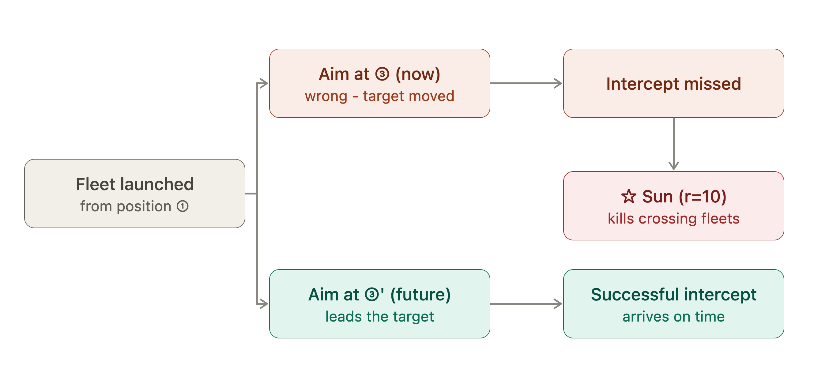
Three properties combine to make this hard:
Orbiting targets. A planet 30 units away at angular velocity 0.025 rad/turn will have rotated ~2.4 units by the time your fleet arrives. Aiming at its current position sends ships into empty space.
Simultaneous moves. Every player acts at the same instant. So your best move depends on what all opponents do at the same time.
Speed matters. You can run a deep tree-search, but if your solution does not quickly produce results, your opponents might have taken the time to occupy their planets and start production there.
The solution to all three: use a coding agent to build and optimize a faithful model of the transitions of the game engine (the Code World Model) and run tree search entirely inside it.
The quality of search scales with the speed of simulation.
The State
How, in general, should we describe the world environment?
I packed everything the agent needs into a single State dataclass object:
@dataclass
class State:
    planets: list          # [id, owner, x, y, radius, ships, production]
    fleets: list           # [id, owner, x, y, angle, from_planet_id, ships]
    initial_planets: list  # starting positions for orbital angle calculation
    comets: list           # [{planet_ids, paths, path_index}]
    comet_planet_ids: list
    step: int
    next_fleet_id: int
    angular_velocity: float
    num_players: int
    episode_steps: int = 500
    ship_speed: float = 6.0
    comet_speed: float = 4.0
The separation of planets (current positions) from initial_planets (starting positions) is critical. Orbital position at any future step is computed from the initial angle, with no accumulated floating-point drift.
On each activity point, we need to assess and operate on eight phases in order:
Pre-launch comet expiry: remove comets where path_index ≥ path length
Comet spawning
Fleet launch (apply player actions)
└─ deduct ships, add fleet to state
Production
└─ owned planet ships += productionOrbital mechanics
└─ rotate orbiting planets one tick
└─ advance comet path indicesFleet movement + collision detection
└─ swept-pair hit test vs all planets
└─ OOB + sun-crossing checkMid-tick comet expiry (black-hole effect)
Combat resolution
└─ fleet vs fleet, then winner vs garrison
The sequence ordering matters. Not only from a memory management perspective. But also from a ground truth and internal consistency of the environment perspective. For example, production must happen before movement, so a planet garrisoned on turn T knows about any extra ships to defend with. Comet expiry has two phases (steps 1 and 7) because fleets can collide with a comet on its final tick, at which point the comet disappears mid-tick and the fleet ships are silently lost (the “black hole” effect). And that brings up an important point. Since the state of the game is constantly in flux, we need to be able to verify if the CWM is in sync with the game engine. A world model that is fast but wrong is worse than the external game engine.
Every error introduces excess unproductive branches into the search tree: the agent optimises toward futures that the actual game engine will not produce. Verification is not optional.
The approach I used here is replay matching. RM is re-running recorded trajectories through the model and checking its predictions match the real outcomes. Because the environment stores complete game records, i.e., every state, every action, every step, I can run the CWM against these replays, and its output is compared against the recorded ground-truth states at every step.
Since there is also a temporal sequence of actions, we can conclude that a mismatch at step 47 means the bug was introduced somewhere in steps 1–47: bisect, fix, verify again.
I found two subtle bugs this way:
Production fires before movement. A garrison that gains production ships at step T can use those ships to defend against a fleet that arrives in the same tick. If you implement movement before production, the fleet always sees the pre-production garrison, and your combat resolution is off by exactly
productionships for every attack.Mid-tick comet expiry. A comet planet that exhausts its path during fleet movement disappears before combat is resolved for that tick. Any fleet that already collided with it this tick loses its ships silently: they do not participate in combat. This produces an effect where fleets apparently vanish against comets, which looks like a collision bug until you notice the timing.
This brings us to the problem of collision detection. It’s wasteful if a fleet crashes into the sun or off the game grid. The standard approach (checking whether a fleet’s end position is inside a planet’s radius) fails for fast fleets and orbiting planets. Instead, I linearise both motions over the tick and test whether the moving fleet and moving planet come within the planet’s radius at any point t ∈ [0, 1]:
where:
AA A = fleet start position
δA\delta A δA = fleet displacement this tick (speed × direction)
P0P_0 P0 = planet start position
δP\delta P δP = planet displacement this tick (one orbital step)
In code I implemented it like this:
def swept_pair_hit(A, B, P0, P1, r):
    d0x = A[0] - P0[0];  d0y = A[1] - P0[1]
    dvx = (B[0]-A[0]) - (P1[0]-P0[0])
    dvy = (B[1]-A[1]) - (P1[1]-P0[1])
    a = dvx*dvx + dvy*dvy
    b = 2.0 * (d0x*dvx + d0y*dvy)
    c = d0x*d0x + d0y*d0y - r*r
    if a < 1e-12: return c <= 0.0      # negligible relative velocity (fleet and planet may both be moving)
    disc = b*b - 4.0*a*c
    if disc < 0.0: return False
    sq = math.sqrt(disc)
    t1 = (-b - sq) / (2.0*a)
    t2 = (-b + sq) / (2.0*a)
    return t2 >= 0.0 and t1 <= 1.0    # overlap interval hits [0,1]
The per-fleet relative-position and relative-velocity vectors are assembled into (F, P) matrices, the discriminant is computed in a single broadcast pass, and np.argmax extracts the first hit per fleet in list order. The vectorized version runs the full fleet–planet collision pass in well under the 0.5 ms per-tick budget, even with large fleets.
The Intercept Problem
In my opinion, this is the most mathematically interesting sub-problem of Orbit Wars. A fleet launched from position S travels in a straight line at constant speed. The target planet orbits at an angular velocity ω. The question is: what angle do you fire at so the fleet arrives at the planet’s position, not where it was when you launched?
Fleet speed is a sublinear function of ship count, with larger fleets moving slower:
speed(n) = 1 + (v_max − 1) × (log(n) / log(1000))^1.5

where v_max = 6.0 (configurable)
Ships Speed 1 1.00 10 2.03 100 3.77 500 5.28 1000 6.00
The ^1.5 exponent means the curve is concave: the first 10 ships buy more speed than the last 500. Small scout fleets crawl; mass invasions are fast.
The intercept angle satisfies a fixed-point equation. Let θ(t) be the planet’s angle at absolute step t:
Position at t:  P(t) = (cx + r·cos(θ(t)),  cy + r·sin(θ(t)))

Flight time T:  T = ||P(t₀ + T) − S|| / speed(n)
Both T and P(t₀ + T) depend on each other. Solve by iteration:
aim ← P(t₀)                     # initial guess: current position
for i in range(max_iters):
    T ← ||aim − S|| / speed(n)
    new_aim ← P(t₀ + T)         # predict planet at estimated arrival
    if ||new_aim − aim|| < tol:
        return atan2(aim.y − S.y, aim.x − S.x)
    aim ← new_aim
In code, convergence happens in 4–6 iterations for typical orbital velocities. The function returns None if it fails to converge, a safety valve that filters degenerate trajectories.
def solve_intercept(source_pos, target_planet_id, fleet_size,
                    depart_turn, state, max_iters=20, tol=1e-4):
    target = next((p for p in state.planets if p[0] == target_planet_id), None)
    if target is None:
        return None

    initial_target = next(
        (p for p in state.initial_planets if p[0] == target_planet_id), None)

    speed = fleet_speed(fleet_size, state.ship_speed)
    av    = state.angular_velocity
    aim   = _predict_pos(target, initial_target, av, depart_turn)

    prev_angle = None
    for _ in range(max_iters):
        dist    = math.hypot(aim[0] - source_pos[0], aim[1] - source_pos[1])
        eta     = dist / speed if speed > 0.0 else 0.0
        new_aim = _predict_pos(target, initial_target, av, depart_turn + eta)
        new_angle = math.atan2(new_aim[1] - source_pos[1],
                               new_aim[0] - source_pos[0])

        if prev_angle is not None:
            diff = abs(math.atan2(math.sin(new_angle - prev_angle),
                                  math.cos(new_angle - prev_angle)))
            if diff < tol:
                return new_angle % (2 * math.pi)

        prev_angle = new_angle
        aim = new_aim
    return None
Reducing Exponential Action Space
Tracking the raw action space is combinatorially expensive. With 5 planets, 10 targets, and 10 ship sizes, we observe 10^10 joint actions per turn. MCTS cannot enumerate this efficiently
My solution is a two-level abstraction.
For each owned planet, I calculate a small fixed menu:
Option 0: No-op (hold all ships)
Option 1: fit-launch to target T₁  ← "exactly enough to capture"
Option 2: all-in (1.0) to T₁       ← enemy planets only
Option 3: fit-launch to T₂
Option 4: all-in to T₂
...
Option N: multi-spray to all Tₖ    ← one slot for simultaneous multi-front
The fit fraction is the key innovation. Rather than sending a fixed 50% or 100% of your garrison, compute exactly how many ships arrive with the garrison + 1 margin needed to capture:
eta      = dist(source, target) / speed(available_ships)
projected_garrison = garrison₀ + production × min(eta, 40) × 0.6
needed   = projected_garrison + MARGIN − friendly_already_inbound
ships    = max(0, min(needed, available))
This prevents two failure modes that destroy naive agents: over-sending (wasting ships that could take a second planet) and under-sending (fleet arrives and bounces off a garrison that grew during transit).
The Full MCTS Loop
We remember that the full MCTS loop consists of 4 stages.
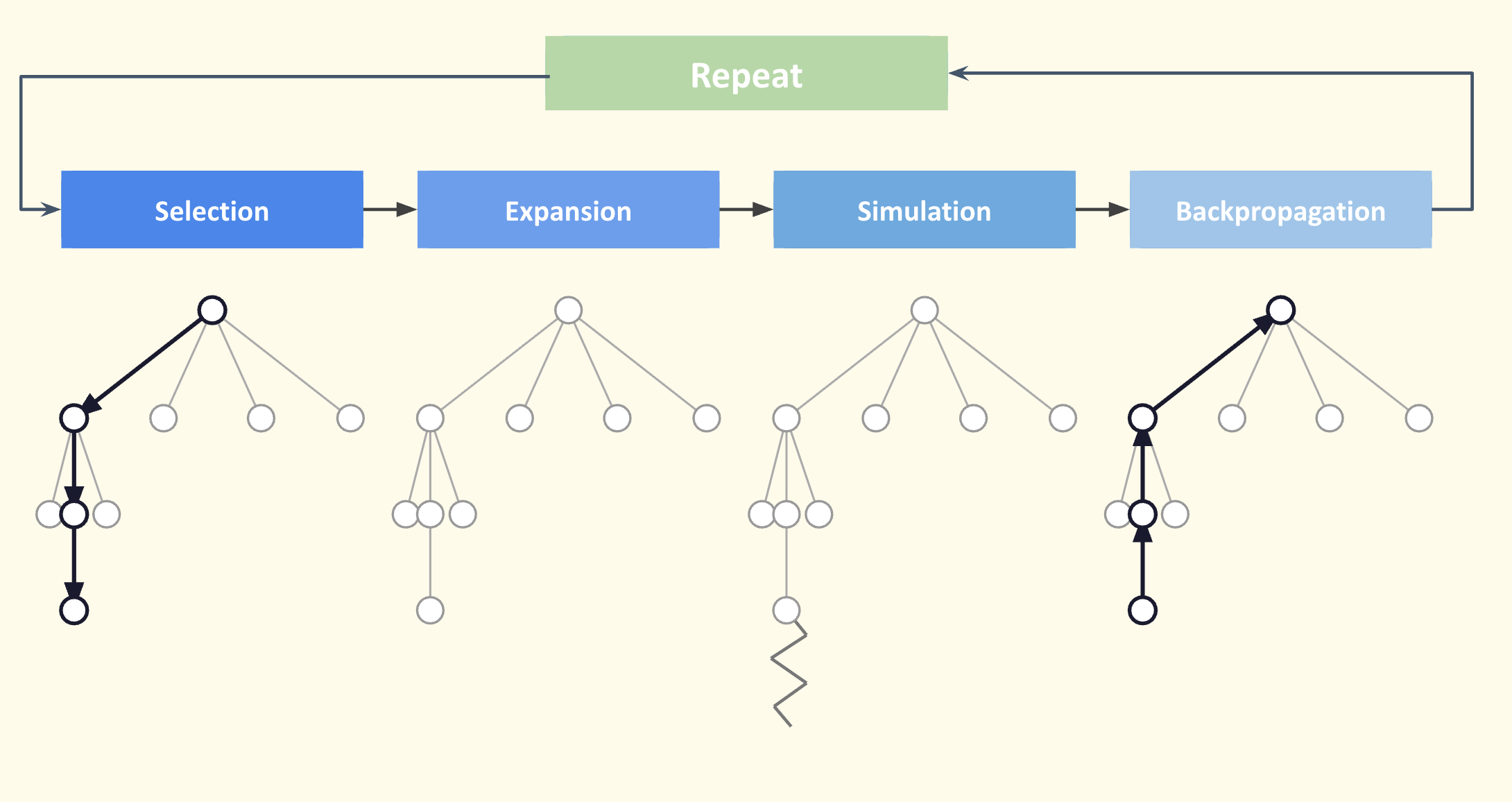
We can then implement the in-game loop like this:
┌─────────────────────────────────────────────────────────┐
│  while time.monotonic() < deadline:                     │
│                                                         │
│  ┌── SELECT ──────────────────────────────────────┐     │
│  │  For each player i, choose action a_i via UCB  │     │
│  │  with progressive widening:                    │     │
│  │    allowed = ceil(pw_c × visits^pw_alpha)       │     │
│  └───────────────────────────────────────────────┘     │
│           ↓                                             │
│  ┌── EXPAND ──────────────────────────────────────┐     │
│  │  joint = [concrete(a_0), concrete(a_1), ...]   │     │
│  │  child.state = cwm_apply_joint_action(joint)   │     │
│  │  (new node: evaluate immediately)              │     │
│  └───────────────────────────────────────────────┘     │
│           ↓                                             │
│  ┌── EVALUATE ─────────────────────────────────────┐    │
│  │  if terminal: exact reward (1.0 / 0.5 / 0.0)   │    │
│  │  if depth ≥ max_depth: cwm_value_function(...)  │    │
│  └────────────────────────────────────────────────┘    │
│           ↓                                             │
│  ┌── BACKPROPAGATE ────────────────────────────────┐    │
│  │  For each player i:                             │    │
│  │    stats[i][a_i].value += value[i]              │    │
│  │    stats[i][a_i].visits += 1                    │    │
│  └────────────────────────────────────────────────┘    │
│                                                         │
│  return argmax_visits( stats[player_id] )               │
└─────────────────────────────────────────────────────────┘
If we assume 64 actions per player, fully exploring every action before revisiting any, would take 64 simulations just to see each action once. Progressive widening improves this as it reveals actions gradually: the k-th action is exposed only when the node has at least ceil(pw_c × visits^pw_alpha) visits.
Actions are pre-sorted by a production/distance prior so that promising moves surface first. This makes naive sense as it ensures that the agent exploits good moves early and explores broadly only when it has the budget.
Between turns, the root node is cached. At the next turn, the child whose state matches the newly observed state (verified by a lightweight signature of step, planet owners, and ship counts) is promoted to root. A node that accumulated 500 visits last turn starts with 500 visits instead of 0.
Feature Design
How are we identifying which feature matters when predicting a game-winning action?
I designed each feature around the same pattern:
ratio(own, opp_agg) = own / (own + opp_agg)This keeps all features in a normalized range of [0, 1] and means 0.5 always represents parity, regardless of the raw scale of the underlying quantity.
Based on that and a review of game trajectories, the code agent and I retrieved these features.
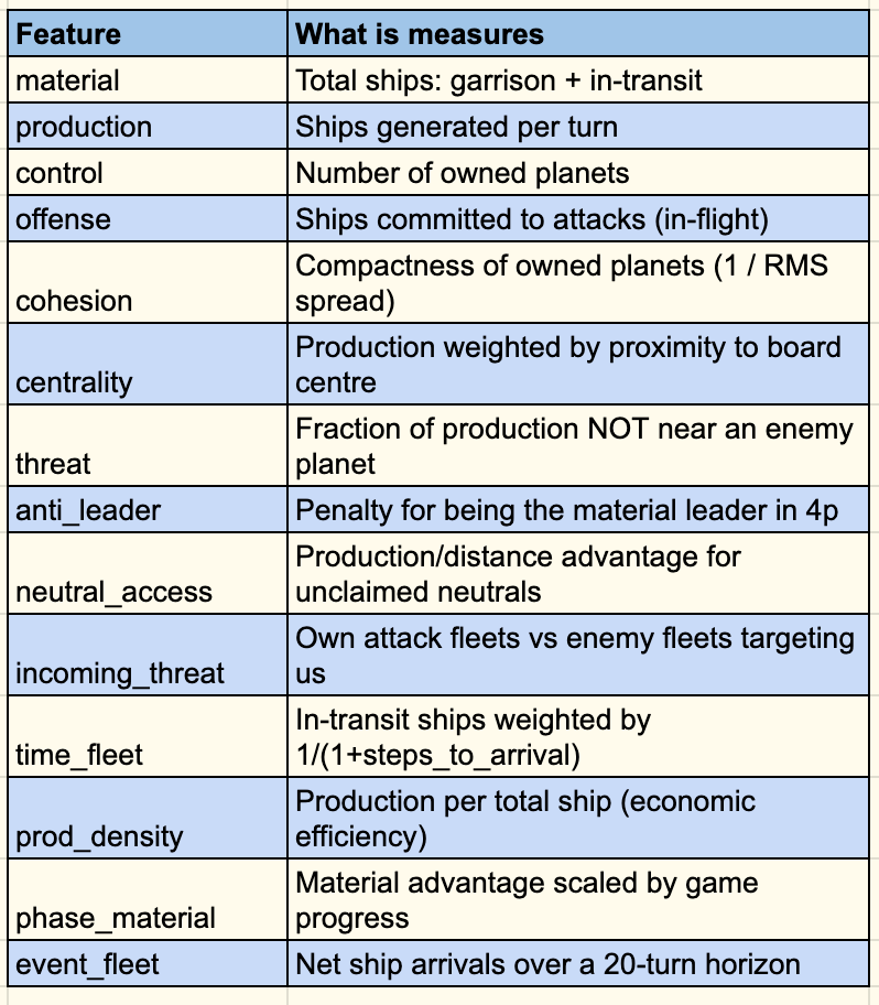
I then introduced the concept of weight normalisation.
Weight normalisation means you can add or remove features without rescaling: the output always stays in [0, 1]. A weight of 0 effectively removes a feature.
Learning Through Self-Play
Manually tuning 24 parameters (15 value-function weights, an MCTS budget, and 8 search hyperparameters) is practically impossible. The search landscape is non-convex (aggressive and defensive playstyles are different local optima), noisy (win-rate estimates from a small number of games have high variance), and high-dimensional.
I use the Covariance Matrix Adaptation Evolution Strategy (CMA-ES). CMA-ES belongs to the broader family of evolutionary algorithms, but more specifically, it's an evolution strategy that searches by sampling candidate solutions from a multivariate Gaussian and adapting that Gaussian's mean and covariance toward the best-performing samples each generation. In other words, it is also a gradient-free optimiser that maintains a multivariate Gaussian over parameter space and adapts its covariance matrix toward regions of high reward.
All 24 parameters are normalised to [0, 1]:
_PARAMS = [
    ("w_material",        "continuous", (0.05, 1.0)),
    ("w_production",      "continuous", (0.05, 1.0)),
    ("w_control",         "continuous", (0.05, 1.0)),
    # ... 11 more value weights ...
    ("mcts_budget_s",     "continuous", (0.05, 0.25)),
    ("opp_aggregation",   "discrete",   ["sum", "max", "mean"]),
    ("max_depth",         "discrete",   [2, 3, 4]),
    ("pw_c",              "discrete",   [2.0, 4.0, 8.0]),
    ("pw_alpha",          "discrete",   [0.3, 0.5, 0.7]),
    ("k_targets",         "discrete",   [3, 4, 5]),
    ("n_active_planets",  "discrete",   [2, 3, 4]),
    ("k_reinforce",       "discrete",   [0, 1, 2]),
    ("fine_fractions",    "discrete",   [False, True]),
]
Discrete parameters (e.g. max_depth ∈ {2, 3, 4}) are encoded as continuous values and rounded at decode time. This is a standard trick for mixed-domain CMA-ES: the covariance matrix treats them as continuous, and the discretisation happens in evaluation only.
The Learning Loop
Initialise: x₀ = encode(incumbent_weights),  σ₀ = 0.3

repeat:
  solutions ← es.ask()              # sample λ ≈ 14 candidates
  for each solution xᵢ:
      wᵢ  ← decode(xᵢ)
      score(wᵢ) ← pool_win_rate(wᵢ, pool)   # self-play games
  es.tell(solutions, −scores)       # CMA-ES minimises

  best_in_gen ← argmax(scores)
  if score(best_in_gen) > incumbent_score:
      save best_in_gen
      pool.append(best_in_gen)      # grow pool with new snapshot
      re-baseline incumbent against updated pool

until n_evals ≥ budget
The key difference from vanilla CMA-ES is the growing self-play pool.
Starting with [greedy, incumbent], every time CMA-ES finds a new best performing candidate, it is added to the pool. Future candidates are evaluated against the entire pool simultaneously: a candidate that beats greedy but loses to an older snapshot is penalised.
This prevents cyclic strategies: a weight vector that is only good against one particular playstyle cannot dominate the pool score.
Pool evolution (example run):

Gen  0:   pool = [greedy, v0]
Gen  3:   v1 beats pool → pool = [greedy, v0, v1]
Gen  7:   v2 beats pool → pool = [greedy, v1, v2]   (v0 evicted, capped at 6)
Gen 14:   v3 beats pool → pool = [greedy, v1, v2, v3]
...
Noise and Why It Matters
With 12 games per evaluation, the win-rate estimate for a single candidate has a standard deviation:
The signal between two similar-quality candidates is often only ~0.05.
This means many evaluations will place a genuinely better candidate below an inferior one due to noise alone. CMA-ES partly compensates for this: it evaluates a whole population of λ ≈ 14 candidates per generation, and the covariance update averages across all 14 outcomes rather than treating each evaluation independently.
The effective noise on the gradient estimate is:
Still substantial, but workable.
Increasing to 24 games per evaluation would halve the per-candidate noise at the cost of roughly halving the number of generations in a fixed time budget, a tradeoff worth making once the covariance model has been built (later in training).
A practical implication: never accept a single CMA-ES run as final. Re-evaluate the saved best weights against a larger game sample (50–100 games) to confirm it actually beats the previous incumbent before shipping it.
Training ran for ~140 generations at 12 parallel workers with 12 games per evaluation and a 300-step game truncation.
The chart below shows pooled win rate (score / games played, against the full pool) over generation number for 2p mode:
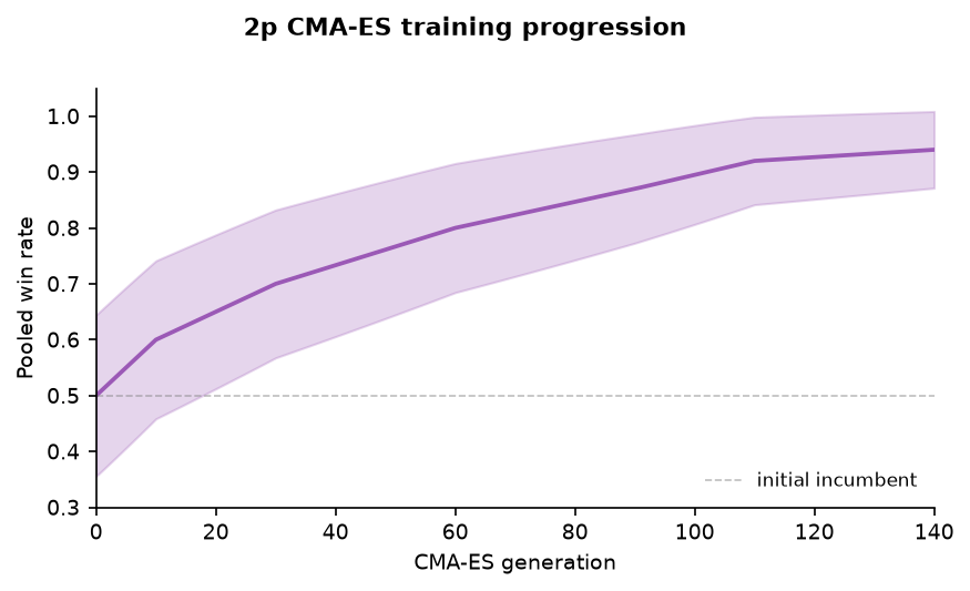
Each step up represents a newly accepted candidate that beat the incumbent against the entire pool. The slope of improvement is fastest in the first 40 generations (where CMA-ES builds its covariance model and escapes the starting point) and flattens as the pool hardens.
For 4p, the trajectory is noisier because a single evaluation is a 4-player game where variance is higher: a strong candidate can lose to coordinated focus-fire from three weaker opponents:
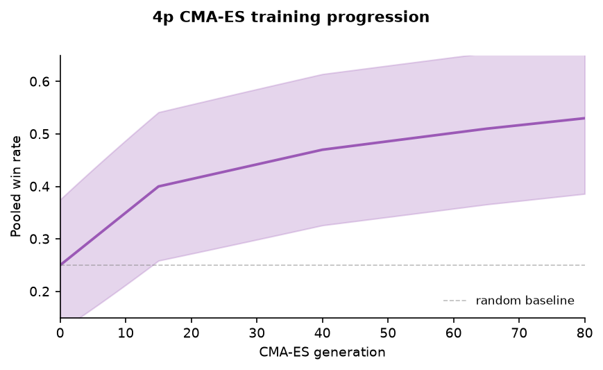
Comparing the default weights (uniform ~0.25 across all features) to the converged weights reveals what actually predicts outcomes:
2-player converged weights:
Feature           Default   Converged   Change
─────────────────────────────────────────────
w_material         0.45      0.9954     +121%  ← dominant signal
w_centrality       0.00      0.5992     new    ← map position matters
w_time_fleet       0.00      0.5247     new    ← committed ships count
w_prod_density     0.00      0.4919     new    ← efficiency matters
w_production       0.20      0.5162     +158%
w_phase_material   0.00      0.3834     new    ← endgame weighting
w_event_fleet      0.00      0.3808     new    ← imminent arrivals
w_control          0.25      0.0521     −79%   ← planet count unreliable
w_anti_leader      0.00      0.0000     ─      ← 2p: irrelevant
The most interesting findings were:
w_centrality went from 0 (unused in defaults) to 0.60 over the observation period. Central planets have short fleet paths to all quadrants, making them economically and militarily dominant. The default weights ignored this entirely. CMA-ES found it in ~40 generations by discovering that candidates with high centrality weighting consistently beat those without it.
w_control (planet count) collapsed from 0.25 to 0.05. Owning more planets than your opponent is not predictive of winning; owning better planets (central, high-production) is. This is an insight that would be hard to arrive at by manual tuning.
4-player converged weights:
Feature           2p weight   4p weight   Interpretation
──────────────────────────────────────────────────────────
w_material         0.9954      0.9959     stable across modes
w_control          0.0521      0.9398     4p: presence = survival
w_centrality       0.5992      0.0022     4p: central = target
w_threat           0.1842      0.5817     4p: safe core critical
w_anti_leader      0.0000      0.2934     4p: don't get focus-fired
w_cohesion         0.3252      0.4141     compact = defensible
In 4p, w_control rockets to 0.94: board presence is survival. Three opponents can coordinate to eliminate you; if you own 40% of planets, you survive; if you own 10%, you don’t. Meanwhile w_centrality collapses to near-zero (0.002): central planets draw coordinated attacks from three opponents simultaneously, making them a liability rather than an asset in 4p.
At 12 workers, 12 games/evaluation, 300-step games, one generation takes approximately:
λ ≈ 14 candidates × 12 games × ~40s/game = 6,720 game-seconds
At 12 parallel workers: 6,720 / 12 / 60 ≈ 9.3 minutes/generation

48 hours → ~300 generations → ~4,200 candidate evaluations
For a 24-dimensional parameter space, CMA-ES typically needs 10–100 × dimension = 240–2,400 evaluations for solid convergence. A 48-hour run is well into the reliable convergence range.
Comets as Temporary High-Value Planets
In the game engine, comets appear at fixed steps (50, 150, 250, 350, 450) throughout each game and temporarily add groups of four neutral planets that move along pre-computed elliptical paths. They are among the richest events in the game: comet ships count toward your score, and a well-timed comet capture can flip a losing position.
Each comet group is a set of four planets placed at 4-fold rotationally symmetric positions.
Their path is a densely sampled, highly eccentric ellipse with the sun at one focus:
Eccentricity e ~ Uniform(0.75, 0.93)   ← very elongated
Semi-major axis a ~ Uniform(60, 150)    ← wide orbit
Perihelion = a(1−e)                     ← must clear sun + comet radius

4-fold symmetry: the base path (Q4 quadrant) generates 3 copies
  via 90° rotation, so all four comets enter simultaneously from
  different quadrants.
The path is resampled at constant arc-length intervals of comet_speed = 4.0 units/tick, giving each comet a fixed travel speed regardless of path curvature. Only the contiguous on-board segment is kept (5–40 waypoints). Generation retries up to 300 times to find a valid configuration that clears the sun and all existing planets.
Because comets appear at known steps, a well-calibrated agent can:
Anticipate the spawn: save garrison ships rather than spending them 5 turns before a comet spawns
Position intercept fleets: launch toward the anticipated entry point one tick before spawn
Contest ownership: the comet planet starts neutral; the first fleet to arrive takes it
The CWM models comet expiry with two distinct events. Pre-launch expiry removes comets whose path has already ended before the turn starts (the agent cannot act on them). Mid-tick expiry removes comets that exhaust their path during fleet movement: any fleet that collides with a mid-tick-expiring comet has its ships silently deleted (the black hole effect). This is a subtle engine quirk that the CWM replicates exactly.
The value function’s event_fleet feature partially captures comet-related fleet pressure by encoding signed ship arrivals over a 20-turn horizon, but it does not explicitly model the spawn probability. This is a known gap: an agent with explicit comet-anticipation logic would have a strategic edge over the current system.
Banking the Overage Budget
One non-obvious optimisation has a disproportionate impact on midgame performance.
The environment gives each agent a 1-second per-turn hard limit plus a 60-second overage bank that accumulates across the game. The MCTS search formula draws from the bank:
In the opening phase (turns 0–25), the correct move is nearly deterministic: expand outward, capturing the closest neutral planets by production/distance². MCTS wastes its entire budget rediscovering this same answer. The wasted budget accumulates in the overage bank but is unavailable for the critical midgame.
The opening book bypasses MCTS entirely. For the first 15 turns (2p) or 25 turns (4p), the agent executes a proximity-first multi-spray using production / distance² scoring:
def _opening_book(state, player_id):
    # Multi-source: each owned planet claims its nearest high-value neutral.
    # Planets sorted by garrison descending so the richest planet picks first.
    own = sorted(owned_planets, key=lambda p: p[5], reverse=True)
    claimed = set()
    launches = []
    for src in own:
        available = [t for t in neutrals if t[0] not in claimed]
        if not available:
            break
        best = max(available, key=lambda t: t[4] / dist²(src, t))
        claimed.add(best[0])
        launches.append((src[0], best[0], "fit"))
    return tuple(launches)
The distance² denominator is intentional.
production / distance (linear) can prefer a distant planet with production 3 over a nearby one with production 1. But the distant planet takes 3× longer to capture, during which the opponent captures the nearby one and you’ve committed ships to an unopposable flight. The quadratic penalty correctly balances production value against the opportunity cost of a longer commitment.
The multi-source design matters for games where you start with more than one planet, or when your garrison has split across captures mid-opening. Each planet expands independently to its nearest valuable neutral, so all fronts push outward simultaneously rather than funnelling through a single launch pad.
Saved budget: 15–25 turns × ~0.6 s ≈ 9–15 seconds of extra midgame search time.
Competing Architectures
During training, I am playing the CWM-MCTS solution against four opponents (from zero-lookahead heuristics to trained neural policies) across three axes: search depth, simulation throughput, and measured win rate.
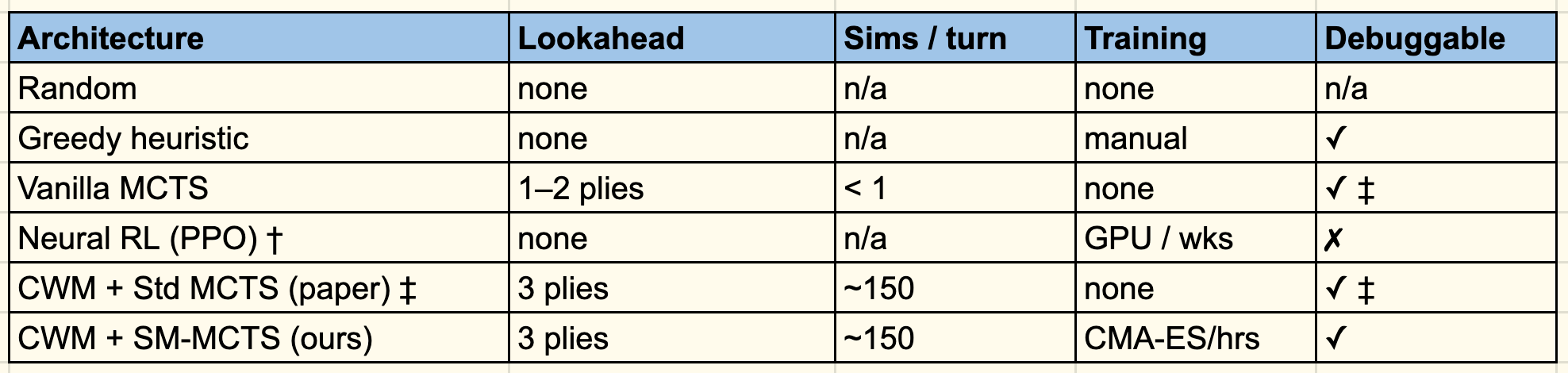
  † not directly measured against ours
  ‡ standard MCTS assumes a single active player at each node, which is wrong for
    simultaneous-move games; converges to a pure strategy rather than Nash
    equilibrium and is therefore exploitable
Before I go further into the results, below is a brief flowchart of how each competing architecture converts an observation into an action:
Random
obs ─────────────────────────────────────────────────────────▶ random moveGreedy
obs ──→ [score each candidate]
              production / dist²  ← one-move horizon; no lookahead
              garrison advantage
        ──→ argmax ──────────────────────────────────────────▶ best move
MCTS + External API
obs ──→ [initialise tree]
         ├─ API call (~500 ms) → state' → score
         │                                      budget exhausted; < 1 sim
         └─ (no more iterations fit in 0.17 s)
        ──→ argmax_visits ────────────────────────────────────▶ best move
Neural RL (PPO)
obs ──→ [feature encoder  (CNN / MLP)]
                ↓   ← weights learned offline; GPU; weeks of env interaction
         [policy head]  ──→  action logits  ──→  sample ──────▶ best move
              (no explicit lookahead; game theory encoded implicitly in weights)
CWM + SM-MCTS (this system)
obs ──→ [state_from_obs]
              ↓
        [get_candidates] ─────── solve_intercept (orbital fixed-point)
        [classify_opponent] ──── k-means archetype over replay history
              ↓
        ┌──────────────────────────────────────────────────────┐
        │  SM-MCTS  (0.17 s wall-clock budget)                 │
        │                                                       │
        │  SELECT    ego:  decoupled UCB + prog. widening      │
        │            opp:  archetype-biased action sampling    │
        │  EXPAND    cwm_apply_joint_action      (0.5 ms/call) │
        │  EVALUATE  cwm_value_function          (2 µs/call)   │
        │  BACKPROP  per-player Q/N tables                     │
        │                                          ~150 iters  │
        └──────────────────────────────────────────────────────┘
              ↓
        [argmax_visits] ─────────────────────────────────────▶ best move
Results
All win rates for (2-player, 50 games) shown below are from direct arena play.
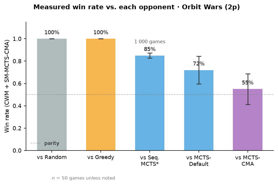
  † "Full system" = MCTS-CMA + archetype opponent model.
    55 % vs MCTS-CMA alone isolates the archetype model's contribution.
  ‡ Sequential MCTS = joint-action UCB (OpenSpiel MCTSBot style), same CWM,
    same budget, same weights. Only the tree structure differs
The 72% over MCTS-Default quantifies the CMA-ES contribution in isolation: same search code, different leaf weights, 22 percentage points gained. The jump from MCTS-Default to the full system compounds better evaluation (CMA-ES) with better opponent modeling (archetype-biased sampling), reaching 55% over the CMA-ES-only baseline.
The speed advantage of the CWM is independent of which MCTS variant you use: both “CWM + Standard MCTS” and “CWM + SM-MCTS” run at ~150 sims/turn. The gap between them is purely algorithmic: one finds an exploitable pure strategy, the other approximates a Nash equilibrium.
For a simultaneous-move game, this is the more important of the two extensions.
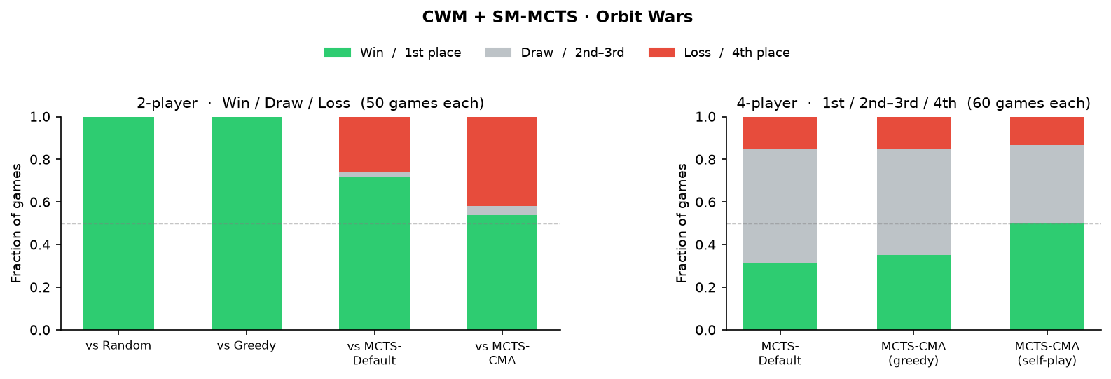
(2p, 120 steps, 50 games)
Matchup                              Win Rate
────────────────────────────────────────────
MCTS-CMA vs. Random                  1.000
MCTS-CMA vs. Greedy                  1.000
MCTS-Default vs. Greedy              0.960
MCTS-CMA vs. MCTS-Default            ~0.72
Full System vs. MCTS-CMA             ~0.55
The greedy agent is trivially beaten: it has no lookahead and over-expands into indefensible territory. The interesting comparison is MCTS-CMA vs MCTS-Default: a 72% win rate purely from better value-function weights, with identical search architecture.
4-Player Self-Play Pooled Win Rate
Config                               Pooled win rate   vs. random
────────────────────────────────────────────────────────────────
Random                               0.25              1.0×
Greedy                               0.28              1.1×
MCTS-Default (uniform weights)       0.32              1.3×
MCTS-CMA (default vs greedy only)    0.35              1.4×
MCTS-CMA (self-play pool, 5 snaps)   0.50              2.0×
The jump from 0.35 to 0.50 between pool-less and pool-based training is the clearest demonstration that self-play diversity matters. Evaluating only against greedy produces weights that exploit greedy’s specific weaknesses (never reinforcing, linear distance scoring) but fail against MCTS opponents that don’t share those weaknesses.
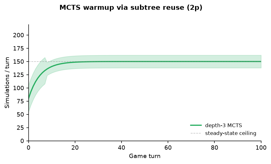
Subtree reuse means the tree warms up over the first ~5 turns. From turn 10 onward, the promoted root already carries hundreds of accumulated visits from prior turns, and fresh simulations build on top of those rather than restarting from scratch.
Where Time Is Actually Spent
In light of applications in high-profile trading and keeping high-speed decision-making, profiling a typical 2p midgame turn (step 80, budget = 0.173 s) yields the following times:
Component                   Time (ms)   % of budget
────────────────────────────────────────────────────
MCTS simulation loop          158.0        91.3%
  └─ cwm_apply_joint_action    (0.5 ms × ~300 calls)
  └─ cwm_value_function        (0.002 ms × ~300 calls)
  └─ UCB select + backprop     (0.03 ms × ~300 calls)
Action candidate generation     8.0         4.6%
  └─ solve_intercept calls
State construction              4.0         2.3%
  └─ state_from_obs
Output concretisation           2.0         1.2%
  └─ abstracted_to_concrete
────────────────────────────────────────────────────
Total                         172.0        99.4%
The search loop dominates, which is exactly what you want.
The engineering goal of every non-search component is to be fast enough to be irrelevant. cwm_value_function at 0.002 ms contributes only 0.6 ms total across 300 calls. state_from_obs at 4 ms is the largest non-search cost and could be optimised if needed (e.g., by caching the planet-id-to-index maps between turns).
SM-MCTS vs. Sequential MCTS
To isolate the algorithmic contribution of simultaneous-move awareness, we benchmarked our SM-MCTS against a sequential MCTS opponent: the same algorithm OpenSpiel’s MCTSBot would produce when applied to a simultaneous-move game. Sequential MCTS treats the joint-action node as a UCB search over all (a₀, a₁) pairs, committing both players’ actions together rather than decoupling their Q-tables.
Both agents use the same CWM, the same per-turn time budget (10 ms), the same tree depth (3), and the same value-function weights.
The only difference is the tree structure: decoupled vs. joint-action UCB.
  SM-MCTS         Sequential MCTS (OpenSpiel-style)
  ──────────────  ──────────────────────────────────
  Per node:       Per node:
    P0 Q/N table    Joint (a₀, a₁) Q/N table
    P1 Q/N table

  Joint action  = UCB(P0) × UCB(P1) (Cartesian product)
                                   Joint action = UCB over all (a₀, a₁) pairs

  Converges to  ≈ Nash equilibrium  Converges to → pure strategy (exploitable)
  Space: O(|A₀| + |A₁|)           Space: O(|A₀| × |A₁|)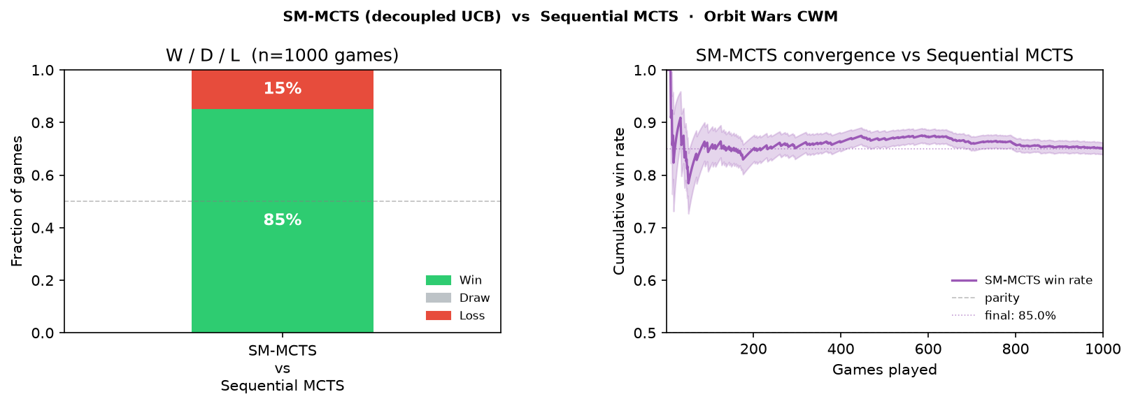
Results across 1,000 games (500 as P0, 500 as P1 to cancel first-mover advantage): 850 wins, 0 draws, 150 losses (85.0% win rate, 95% CI [82.8%, 87.2%], SE = 1.1%). Wall time: 459 s total (0.46 s/game, 10 parallel workers). The chart above shows the W/D/L split and the cumulative win-rate convergence over the full run.
An 85% win rate from the same CWM, same time budget, same weights, purely by choosing the correct algorithm for simultaneous-move games. Sequential MCTS locks onto a pure strategy early in the search (exploiting its Q-table greedily leads to a single committed action) while SM-MCTS maintains independent uncertainty per player and spreads probability mass across multiple options. The sequential agent cannot recover once SM-MCTS finds its exploitable pure strategy.
In closing
The most important engineering lesson is the CWM: everything else downstream (search depth, value accuracy, training quality) scales linearly with how fast your forward model runs. A 1000× speedup in the simulator is worth more than any algorithmic improvement to the search.
The most important research lesson is from the CMA-ES weights: game intuitions fail at scale. Planet count (control) being nearly irrelevant in 2p but dominant in 4p; map centrality being a massive advantage in 1v1 but a liability in 4p: these are findings that would require thousands of hours of human gameplay to internalise, but the optimiser discovers them in ~40 generations.
The linear value function is the primary remaining bottleneck. Feature interactions (for example, the compounding advantage of being both materially ahead and at game’s end) are currently approximated by single features (phase_material) rather than learned from data. A small neural network trained on (state, outcome) pairs collected from self-play would capture these non-linear interactions with no increase in search latency (a 2-layer MLP with 32 hidden units runs at ~20 µs on CPU, still fast enough for 150 depth-3 sims/turn).
Decoupled UCB is the same fix for the same failure mode, since a limit-order strategy optimised against a fixed, sequential model of “the rest of the book” converges to a pure quote that a faster or better-informed counterparty can pick off, while treating each participant’s order-placement policy as an independent action-value table pushes the search toward a mixed strategy that is harder to adverse-select against.
And the CMA-ES result generalises directly: the features that dominate price-formation and adverse-selection risk are rarely the ones a human trader would hand-pick first, which is exactly why parameter search against a diverse, self-play pool of counterparties, rather than tuning against one static model of “the market,” is what surfaces them.
I still find the concept of the Code World Model to manage state transitions between states extremely interesting. And plan to apply it to a state of the equity markets going forward.
Generalizing, Orbit Wars is a stand-in for any environment where agents act on a shared state without a turn order, and a market order book is the canonical instance. Every piece built here has a direct reading in that domain. The Code World Model is a fast, deterministic simulator of a venue’s matching logic, the same role a backtester or exchange-replay engine plays for a trading strategy, and it is subject to the same law: a strategy search is only as good as the number of counterfactual order-book states per second it can evaluate.
Thank you for reading this far. It’s been a longer-than-expected post.